文章快速检索     高级检索
  华东师范大学学报(自然科学版)  2019 Issue (2): 32-48  DOI: 10.3969/j.issn.1000-5641.2019.02.004
0

引用本文  

哈达德, 葛磊. 递归加权科赫网络中平均的齐次与非齐次加权接收时间[J]. 华东师范大学学报(自然科学版), 2019, 2019(2): 32-48. DOI: 10.3969/j.issn.1000-5641.2019.02.004.
ALHADDAD Mansour A. A., MOHAMMAD Gareeb. Average homogeneous and non-homogeneous weighted receiving time in recursive weighted Koch networks[J]. Journal of East China Normal University (Natural Science), 2019, 2019(2): 32-48. DOI: 10.3969/j.issn.1000-5641.2019.02.004.

通信作者

葛磊, 男, 叙利亚, 博士研究生, 研究方向为分形几何.E-mail:silver_man321@hotmail.com

文章历史

收稿日期:2017-07-17
Average homogeneous and non-homogeneous weighted receiving time in recursive weighted Koch networks
ALHADDAD Mansour A. A. , MOHAMMAD Gareeb     
School of Mathematical Sciences, East China Normal University, Shanghai 200241, China
Abstract: In this paper, we introduce the recursive homogeneous weighted Koch network model for real systems with a scaling factor t ∈ (0, 1) and the non-homogeneous model with scaling factors t, s∈ (0, 1) or t, r, s ∈ (0, 1). These models were constructed using the recursive division method and motivated by experimental study of aviation networks and metabolic networks. As a process of fundamental dynamics, we study the recursive homogeneous and non-homogeneous weighted Koch networks with a random walk; for all steps, the walker who is starting from an existing node moves uniformly to one of its nearest neighbors Γ(j) lying on the layers $L_\ell, \ell=0,1,\cdots,m$. In order to study homogeneous and non-homogeneous models, the recursive division method and singular value decomposition were used to calculate the sum of the mean weighted longest paths (MWLP) for all nodes absorbed at the target node placed in one of the merging nodes {pi:i=1, 2, 3}. Finally, in a large network, the average weighted receiving time (AWRT) for homogeneous and nonhomogeneous models grows sub-linearly with the network's order.
Keywords: homogeneous weighted Koch network    non-homogeneous weighted Koch network    recursive division method    average weighted receiving time    
递归加权科赫网络中平均的齐次与非齐次加权接收时间
哈达德 , 葛磊     
华东师范大学 数学科学学院, 上海 200241
摘要:本文介绍用递归分割方法得到的实数系统上递归的齐次和非齐次的加权科赫网络模型,其主要是受机场网络和代谢网络的经验观测的启发.其中对于齐次模型,它依赖比例因子t ∈(0,1);对非齐次的模型,我们通常取不同的比例因子tstrs∈(0,1).作为基本的动力学过程,我们研究递归的齐次与非齐次的加权科赫网络的随机行走,即每一步后都将一致移动到任意一个其位于边界$L_\ell, \ell=0,1,\cdots,m$,上的领域Γ(j)中.为了更方便研究齐次与非齐次模型,我们会再次用到递归分割法以及奇异值分解法来计算所有的节点与目标节点之间最长路径的平均加权(MWLP)的总和,其中目标节点是合并节点{pii=1,2,3}中的某个节点.最终,在庞大的网络中,平均的齐次与非齐次加权接收时间将关于网络秩序次线性.
关键词齐次加权科赫网络    非齐次加权科赫网络    递归分割法    平均加权接收时间    
0 Introduction

Networks provide a mathematical structure for the analysis of natural and man-made systems. We need networks in scientific communities and they exist in nature in many complex systems; these system can be represented as random graphs or directed networks[1] where the nodes are the components that represent the system, while the edges link connecting elements and stand for the interactions between the nodes. Typical examples include river networks, scientific collaboration networks, highway networks, the worldwide airport network, metabolic networks, etc[2-6]. A fractal network is a geometric form which is self-similar and has fractional dimension. Meifeng Dai et al. introduced the box dimension of weighted fractal networks[7-8].

Recently, fractals have attracted growing attention in mathematics, physics, and other scientific studies. Biologists use them in examining certain dynamical diseases, and mathematicians use them in research projects, owing to the striking beauty intrinsic in their structures and the increasing impact of the fractals concept. Hence, it is important to combine weighted networks with the fractals concept, which we refer to hereinafter as weighted fractal networks[9-10]. In [11], the concept of mean first-passage time on a Koch network was proposed. Long Li et al. studied the scaling of mean first-passage time of a family of small-world treelike networks created by two parameters[12]. Inspired by Koch fractals, researchers proposed a family of actual networks called Koch networks and weighted tetrahedron Koch networks[13-15].

Motivated by airport networks, metabolic networks, and by the recursive division method[16], we construct the recursive homogeneous and non-homogeneous weighted Koch networks in which each edge's weight in every triangle depends on the scaling factor t∈ (0, 1) for homogeneous model and on different scaling factors t, s ∈ (0, 1) or t, r, s ∈ (0, 1) for the non-homogeneous model. In this paper, random walk on a family of homogeneous and non-homogeneous weighted Koch networks was studied. Based on the definition of the average weighted longest path (AWLP), we define the average weighted receiving time (AWRT). In this model, the walker at each step starts from its beginning node and moves uniformly to one of its neighbors. Moreover, the AWLP, in the infinite limit of the network order, only depends on the sum of scaling factors t, r, s∈(0, 1). We should mention that we only study a specific family of non-homogenous fractal hierarchical structures and non-homogenous weighted Koch networks, as mentioned by Meifeng Dai et al. in [17-18]. Our results show that in a large network, the AWRT grows as a constant of the network order when the k-th generation goes to infinity, represented by $\theta \left( t \right) = \frac{{2\left( {t + 2} \right)}}{{3\left( {1 - t} \right)}}$, 0 < t < 1, for the homogeneous model, and $\theta \left( {t, s} \right) = \frac{{16\left( {t + 2} \right)\left( {s + 2} \right)}}{{3\left( {16 - 8s\left( {t + 1} \right)} \right)}}$, 0 < t, s < 1, for the non-homogeneous model.

1 Homogenous weighted Koch networks created by the recursive division method for scaling factor t

In this section, our goal is to construct recursive homogeneous weighted Koch networks. In these networks, the topology of every equilateral triangle has the same weight on its three edges. For convenience, we describe the model using the recursive division method to define recursive homogeneous weighted Koch networks. Let us fix a positive real number t∈ (0, 1), such that the steps of constructing recursive homogeneous weighted Koch networks for all generations k=0, 1, 2, 3, ..., n-1, n, n+1 are as follows.

Step 1 Given an initial network G(0) (i.e., G0), G0 consists of three merging nodes L0={pi:i=1, 2, 3} and three edges linking these nodes with a unit weight forming equilateral triangle as shown in Figure 1.
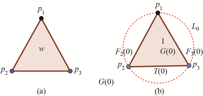
图 1 (a) w represents three edges with weight w in a triangle; (b) G0 (i.e., G(0)) with w=1 Fig.1 (a) w represents three edges with weight w in a triangle; (b) G0 (i.e., G(0)) with w=1

Step 2 Let G0(i), i=1, 2, 3, be three copies of G0, whose weighted edges have been scaled by a factor 0 < t < 1. Let us denote by {pii:i=1, 2, 3}, the node in G0(i) that is the image of the node initially labeled piG0. G(1) is obtained by amalgamating three copies G0(i), i=1, 2, 3, and G0 by merging three pairs of pii and pi, i=1, 2, 3, respectively, into a new single node which are then the merging nodes {pi:i=1, 2, 3} ({1, 2, 3} for short) of G(1), as shown in Figure 2(a).
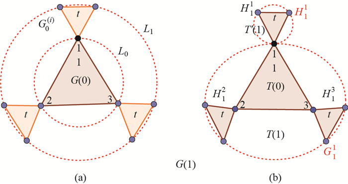
图 2 (a) The construction of G(1) as layers; (b) G(1) is regarded as the merging of H11 and G11 Fig.2 (a) The construction of G(1) as layers; (b) G(1) is regarded as the merging of H11 and G11

For the convenience of constructing of G(2), G(1) can be regarded as the merging of H1i and G1i, i=1, 2, 3, whose connection nodes are {1, 2, 3}, respectively, as shown in Figure 2(b). From the self-similarity of G(1), G(1) can be regarded as four groups, sequentially denoted as G1(0), G1(1), G1(2) and G1(3).

Step 3 Let G1(i) be the copy of G1i, i=1, 2, 3, whose weighted edges have been scaled by a factor 0 < t < 1, and let Q1(i)=G1(i)H1i, i=1, 2, 3, where G1(i)H1i={pii, i=1, 2, 3, {pii:i=1, 2, 3} is the image of the initially labeled node {pi:i=1, 2, 3}. G(2) is obtained by amalgamating three groups Q1(i), i=1, 2, 3, and G(1) by merging three pairs of piiQ1(i) and piG(1), i=1, 2, 3, respectively, into a new single node which are then the merging nodes {pi:i=1, 2, 3} ({1, 2, 3} for short) of G(2), as shown in Figure 3(a).

图 3 (a) The construction of G(2) as layers; (b) G(2) is regarded as the merging of H21 and G21 Fig.3 (a) The construction of G(2) as layers; (b) G(2) is regarded as the merging of H21 and G21

For the convenience of construction of G(3), G(2) can also be regarded as the merging of H2i and G2i, i=1, 2, 3, whose connection nodes are {1, 2, 3}, respectively, as shown in Figure 3(b). From the self-similarity of G(2), G(2) can be regarded as four groups, sequentially denoted as G2(0), G2(1), G2(2) and G2(3).

Step n A large network of order k=n+1 is obtained as follows. Firstly, for the convenience of constructing G(n+1), G(n) can be regarded as the merging of Hni and Gni, whose connection nodes are {1, 2, 3}, respectively, as shown in Figure 4(b).

图 4 (a) The construction of G(n) as layers; (b) G(n) is regarded as the merging of Hni and Gni Fig.4 (a) The construction of G(n) as layers; (b) G(n) is regarded as the merging of Hni and Gni

From the self-similarity of G(n), G(n) can be regarded as four groups, sequentially denoted as Gn(0), Gn(1), Gn(2) and Gn(3). One group is Gn(0)=G0-{pi:i=1, 2, 3}; then G(n)-Gn(0) consists of the same three disjoint groups Gn(i), i=1, 2, 3, whose merging node is linked to the corresponding initial merging node pi of G0. Let Gni=(G(n)-Hni)∪ {pi, i=1, 2, 3, then HniGni={pi, i=1, 2, 3.

Secondly, let Gn-1(i) be the copy of Gn-1i, i=1, 2, 3, whose weighted edges have been scaled by a factor 0 < t < 1, and let Qn-1(i)=Gn-1(i)Hn-1i, i=1, 2, 3, where Gn-1(i)Hn-1i={pii, i=1, 2, 3, {pii:i=1, 2, 3} is the image of the initially labeled node {pi:i=1, 2, 3}.

Finally, G(n) is obtained by amalgamating three groups Qn-1(i), i=1, 2, 3, and G(n-1) by merging three pairs of piiQn-1(i) and piG(n-1), i=1, 2, 3, respectively, into a new single node which are then the merging nodes {pi:i=1, 2, 3} ({1, 2, 3} for short) of G(n), as shown in Figure 4(a). Hence, a recursive homogeneous weighted Koch network created by the recursive division method was obtained.

Now, we can easily get some basic quantities, which are needed for this paper. We denote by $\varOmega$ the set of all nodes of $G(k)$ divided into three disjoint groups $\varOmega_i \subset \varOmega, i=1, 2, 3$, and we will decompose the set of all nodes $\varOmega$ into layers $L_\ell, \ell=0, 1, \cdots, m$; hence, we have $\varOmega=\bigcup_{\ell=0}^{m} L_\ell$ with a disjoint union, so that for all nodes $j\in \varOmega$ there exists a unique $i\in \{1, 2, 3\}$ such that $j\in \varOmega_i$. Let $\ell$ be the minimum number of edges linking the connecting node $j$ to node $i$; thus the node $j\in L_\ell$ and by this way each layer $L_\ell, \ell=1, \cdots, m$, is defined. Let us fix iteration $k\geq 1$ for $G(k)$; then the number of all nodes $N_{L_\ell}(k)$ in the layers $L_\ell, \ell=0, 1, \cdots, m$, is defined by the number of boundary points of the disjoint layers, i.e., $N_{L_\ell}(k)=\sum_{\ell=0}^{m} N_{L_\ell}$ for iteration $k\geq 1$, while the number of nodes in the last layer $L_m$ is $N_{L_m}=2^m N_{L_0}$, where $N_{L_0}=3$ is the number of the nodes in the initial layer $L_0$. The number of triangles $L_{\triangle}(k)$ presented at iteration $k=0, 1, 2, 3, \cdots, n$ is $L_{\triangle}(k)=4^k$. Then, the number of edges is equal to three times the number the triangles in $G(k)$, i.e., $E_k=3L_{\triangle}(k)=3\times 4^{k}$. Similarly, the number of nodes generated at iteration $k=1, 2, 3, \cdots, n$ is six times the number of triangles in $G(k-1)$, i.e., $L_{\nu}(k) =6L_{\triangle}(k-1)=6\times 4^{k-1}$. Hence, the number of all nodes in $G(k)$ is the sum of the numbers of nodes generated at iteration $k=0, 1, 2, 3, \cdots, n$, i.e.,

$ \begin{equation} N_k=\sum\limits_{i=0}^{k}L_{\nu}(i)=2\times 4^k+1. \end{equation} $ (1.1)
2 Average weighted receiving time for scaling factor t

In this section, we will explicitly determine the average homogeneous weighted receiving time (AHWRT) $\langle T \rangle_k$; in our result, we show how $\langle T \rangle_k$ scales with the generation of a large network order. Our purpose is to work on a particular stage in $G(k)$ with a trap placed on one of the merging nodes $\{p_i:i=1, 2, 3\}= L_0$. The process is a random walk, i.e., at each step, the walker starts from its current node $j$ in any layer $L_\ell, \ell=1, \cdots, m$, and moves uniformly to one of its neighbors $i\in \Gamma(j)$ belonging to the previous layer $L_{\ell-1}$. For convenience, let us denote the three merging nodes $\{p_i:i=1, 2, 3\}\in G(k)$ by $\{1, 2, 3\}$ and other nodes $\{p_j:j=4, 5, \cdots, N_k\}\in G(k)$ by $\{4, 5, \dots, N_{k-1}, N_k\}$.

The mean weighted longest paths (MWLPs) is the expected first arriving weighted time for the walker starting from a source node to a given target node in the layer $L_0$. Let $F_{j}(k)$ be the mean weighted longest paths for a walker starting from node $j\in L_\ell, \ell=1, \cdots, m$, to a given target node (trap) located at $i=1$ in the layer $L_0$ of $G(k)$. Note that the models presented here are directed graphs; in this case, the walker who is moving from its current layer $L_\ell$ to its previous layer $L_{\ell-1}$ can not go back again over each step.

From the construction of the homogeneous graph $G(k)$ of a large network, the graph $G(k)$ can be regarded as the union of two groups $H_k^1$ and $H_k^{2, 3}$ (i.e., $H_k^2\cup H_k^3$) which are merging at a node located in trap 1. In the group $H_k^1$ from the above definition of $F_j(k)$ and by the recursive division method for any $j\in H_k^1$, the recurrence formula of $F_j(k)$ can be obtained as $F_j(k)=2t^k+2t^{k-1}+\cdots+2t$; then we have

$ \begin{equation} F_j(k)=\dfrac{2t(t^k-1)}{t-1}, \forall j\in L_\ell, L_\ell \in H_k^1, \ell=1, \cdots, m, k=1, \cdots, n. \end{equation} $ (2.1)

Similarly, in the group $H_k^{2, 3}$ from the above definition of $F_j(k)$ and by recursive division method for any $j\in H_k^{2, 3}$, the recurrence formula of $F_j(k)$ can be obtained as $F_j(k)=2t^k+2t^{k-1}+\cdots+2t+2$; then we have

$ \begin{equation} F_j(k)=\dfrac{2(t^{k+1}-1)}{t-1}, \forall j\in L_\ell, L_\ell \in H_k^{2, 3}, \ell=0, 1, \cdots, m, k=0, 1, \cdots, n. \end{equation} $ (2.2)

Here we denote by $T^\prime(k)$ the sum of (MWLPs) for all nodes in $H_k^1$ absorbed at the trap located at the merging node $p_1\in L_0$ of $G(k)$, i.e., $T^\prime(k)=\sum_{j\in H_k^1\setminus\{1\}}F_j(k)$, and denote by $T(k)$ the sum of (MWLPs) for all nodes in $G_k^1=H_k^{2, 3}$ absorbed at the trap located at the merging node $p_1\in L_0$ of $G(k)$, i.e., $T(k)=\sum_{j\in H_k^{2, 3}\setminus\{1\}}F_j(k)$; then we denote by $T_{\rm tot}(k)$ the sum of MWLPs for all nodes in $G(k)=H_k^1\cup H_k^{2, 3}$ absorbed at the trap located at the merging node $p_1\in L_0$ of $G(k)$, i.e.,

$ \begin{equation} T_{\rm tot}(k)=T^\prime(k)+T(k)=\sum\limits_{j=2}^{N_k}F_j(k). \end{equation} $ (2.3)

Now, $\langle T \rangle_k$ is the average homogeneous weighted receiving time (AHWRT), which is defined as the average of $F_j(k)$ over all starting nodes $j\in G(k)=H_k^1\cup H_k^{2, 3}$, where $H_k^1\cap H_k^{2, 3}=\{1\}$ other than the trap at $G(0)$; then we have

$ \begin{equation} \langle T \rangle_k=\dfrac{T_{\rm tot}(k)}{N_k-1}. \end{equation} $ (2.4)

Thus, the problem of determining $\langle T \rangle_k$ is reduced to finding $T_{\rm tot}(k)$. By the construction of $G(k)$, $G(k)$ can also be regarded as merging of $H_k^1$ and $G_k^1$ (i.e., $H_k$ and $G_k$ for short), whose merging node is $p_1\in L_0$. Note that here we will set $H_k^{2, 3}=H_k^2 \cup H_k^3$ and $G_k^{(2, 3)}=G_k^{(2)} \cup G_k^{(3)}$ for all $k=1, 2, \cdots, n$.

2.1 Recurrence formula of $T_{\rm tot}(k)$ for scaling factor t

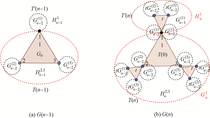
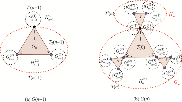
For a large network graph $G(k)$, we can obtain the recursive formulas of $T^{\prime}(k)$ and $T(k)$ by transition from $G(n-1)$ to $G(n)$. The group $H_n^1$ of the graph $G(n)$ consists of the union of three disjoint groups $G_{n-2}^{(1)}, G_{n-2}^{(1)}$ and $G_{n-1}^{(1)}$; then $H_n^1=G_{n-2}^{(1)}\cup G_{n-2}^{(1)}\cup G_{n-1}^{(1)}$, where $G_{n-1}^{(1)}=tT(n-1)$ and $G_{n-2}^{(1)}=T^{\prime}(n-1)$. From the definition of $T^{\prime}(n)$, we obtain

$ \begin{equation} T^{\prime}(n)=2T^{\prime}(n-1)+tT(n-1). \end{equation} $ (2.5)

The group $H_n^{2, 3}$ of the graph $G(n)$ consists of the union of three disjoint groups $2tG_{n-2}^{(1)}, tG_{n-2}^{(2, 3)}$ and $2G_{n-2}^{(2, 3)}$; then $H_n^{2, 3}=2tG_{n-2}^{(1)} \cup tG_{n-2}^{(2, 3)} \cup 2G_{n-2}^{(2, 3)}$. These three groups are obtained as $2tG_{n-2}^{(1)}=2tT^\prime(n-1)+\frac{2}{3}(2t+2)N_{n-1}$, $tG_{n-2}^{(2, 3)}=tT(n-1)+2(\frac{2}{3}N_{n-1})$ and $2G_{n-2}^{(2, 3)}=2T(n-1)-4$; from the definition of $T(n)$, we obtain

$ \begin{equation} T(n)=2tT^{\prime}(n-1)+(t+2)T(n-1)+\dfrac{4}{3}tN_{n-1}+\dfrac{8}{3}N_{n-1}-4. \end{equation} $ (2.6)

See Figure 5. If we fix $k=n$, we can rewrite Eq (2.5) and Eq (2.6) in the form

$ \begin{equation} K_n=AK_{n-1}+\alpha(n), \end{equation} $ (2.7)
图 5 (a) The construction of $G(n-1)$; (b) The construction of $G(n)$ Fig.5 (a) The construction of $G(n-1)$; (b) The construction of $G(n)$

where $K_n= \begin{pmatrix} T^\prime(n) \\T(n)\end{pmatrix}$, $A= \begin{pmatrix} 2&t \\ 2t&t+2 \end{pmatrix}$, $\alpha(n)= \begin{pmatrix} 0 \\a_n \end{pmatrix}$ and $a_n=\frac{4}{3}tN_{n-1}+\frac{8}{3}N_{n-1}-4$.

We can solve Eq (2.7) inductively to get

$ \begin{equation} K_n=A^nK_{0}+\sum\limits_{i=1}^{n}A^{n-i}\alpha(i). \end{equation} $ (2.8)

Now by using singular value decomposition in this work, we seek to find the eigenvalues and the eigenvectors of the matrix $A_{2\times2}$ which represents a linear transformation. For this matrix, there are two eigenvalues equivalent to the two roots of the equation $\lambda^2-(\textrm{tr}A)\lambda+\textrm{det}A=0$; then we have $\lambda_1=2t+2$ and $\lambda_2=-t+2$. Thus, we get two non-zero eigenvectors satisfying $Av_i=\lambda_iv_i, i=1, 2$, $v_1=\begin{pmatrix} 2t \\4t \end{pmatrix}$ and $v_2=\begin{pmatrix} 2t \\-2t \end{pmatrix}$ corresponding to $\lambda_1$ and $\lambda_2$, respectively. So we can rewrite the matrix $A$ as $A=V \Sigma V^{-1}$, where $V= \begin{pmatrix} 2t&2t \\ 4t&-2t \end{pmatrix}$, $\Sigma= \begin{pmatrix} 2t+2&0 \\ 0&-t+2 \end{pmatrix}$ and $V^{-1}=\frac{-1}{12t^2} \begin{pmatrix} -2t & -2t \\ -4t&2t\end{pmatrix}$; then we have

$ A^{n}= \begin{pmatrix} 2 & t \\ 2t & t+2 \end{pmatrix}^{n} = \begin{pmatrix} \dfrac{1}{3}(2t+2)^{n}+\dfrac{2}{3}(-t+2)^{n} & \dfrac{1}{3}(2t+2)^{n}-\dfrac{1}{3}(-t+2)^{n} \\[3mm] \dfrac{2}{3}(2t+2)^{n}-\dfrac{2}{3}(-t+2)^{n} & \dfrac{2}{3}(2t+2)^{n}+\dfrac{1}{3}(-t+2)^{n} \end{pmatrix}. $ (2.9)

By using $K_0= \begin{pmatrix} T^\prime(0) \\ T(0)\end{pmatrix}=\begin{pmatrix} 0 \\ 4\end{pmatrix}$ for the initial network and from Eq (2.9), we obtain

$ A^nK_0= \begin{pmatrix} \dfrac{4}{3}(2t+2)^{n}-\dfrac{4}{3}(-t+2)^{n}\\[3mm] \dfrac{8}{3}(2t+2)^{n}+\dfrac{4}{3}(-t+2)^{n} \end{pmatrix}, $

and

$ \sum\limits_{i=1}^{n}A^{n-i}\alpha(i)= \begin{pmatrix} \dfrac{1}{3}\sum\limits_{i=1}^{n}(2t+2)^{n-i}a_i- \dfrac{1}{3}\sum\limits_{i=1}^{n}(-t+2)^{n-i}a_i\\[3mm] \dfrac{2}{3}\sum\limits_{i=1}^{n}(2t+2)^{n-i}a_i+ \dfrac{1}{3}\sum\limits_{i=1}^{n}(-t+2)^{n-i}a_i \end{pmatrix}. $

From Eq (2.8), we get

$ K_n\!=\! \begin{pmatrix} T^\prime(n) \\ T(n) \end{pmatrix} \!=\!\begin{pmatrix} \dfrac{4}{3}((2t+2)^{n}-(-t+2)^{n})+\dfrac{1}{3}\left(\sum\limits_{i=1}^{n}(2t+2)^{n-i}a_i-\sum\limits_{i=1}^{n}(-t+2)^{n-i}a_i\right) \\[3mm] \dfrac{4}{3}(2(2t+2)^{n}+(-t+2)^{n})+\dfrac{1}{3} \left(2\sum\limits_{i=1}^{n}(2t+2)^{n-i}a_i+\sum\limits_{i=1}^{n}(-t+2)^{n-i}a_i\right) \end{pmatrix}; $

then we obtain the formula of $T^\prime(n)$ and $T(n)$ as follows

$ \begin{equation} T^\prime(n)=\dfrac{4}{3}\left((2t+2)^{n}-(-t+2)^{n}\right)+\dfrac{1}{3}\left(\sum\limits_{i=1}^{n}(2t+2)^{n-i}a_i-\sum\limits_{i=1}^{n}(-t+2)^{n-i}a_i\right) \end{equation} $ (2.10)

and

$ \begin{equation} T(n)=\dfrac{4}{3}\left(2(2t+2)^{n}+(-t+2)^{n}\right)+ \dfrac{1}{3}\left(2\sum\limits_{i=1}^{n}(2t+2)^{n-i}a_i+\sum\limits_{i=1}^{n}(-t+2)^{n-i}a_i\right). \end{equation} $ (2.11)

By the definition of $T_{\rm tot}(n)$, we can write $T_{\rm tot}(n)$ as

\begin{equation*} T_{\rm tot}(n)= 4(2t+2)^{n}+\sum_{i=1}^{n}(2t+2)^{n-i}a_i, \end{equation*}

where $a_i=\frac{4}{3}tN_{i-1}+\frac{8}{3}N_{i-1}-4$ and $N_{i-1}=2\times 4^{i-1}+1$; then $a_i=\frac{2}{3}(t+2)4^i+\frac{4}{3}(t-1)$ and we have

$ \begin{equation*} T_{\rm tot}(n)= 4(2t+2)^{n}+\dfrac{2}{3}\left(t+2\right)\left(\dfrac{2((2t+2)^n-4^n)}{t-1} \right)+\dfrac{4}{3}\left(t-1\right) \left(\dfrac{(2t+2)^n-1}{2t+1}\right). \end{equation*} $

Then for any $k=0, 1, 2, \cdots, n$, we get

$ \begin{equation} T_{\rm tot}(k)= \dfrac{12t^2(2t+2)^k}{(t-1)(2t+1)}-\dfrac{4^{k+1}(t+2)}{3(t-1)}- \dfrac{4(t-1)}{3(2t+1)}. \end{equation} $ (2.12)
2.2 Formula of $\langle T \rangle_k$ for scaling factor t

Finally, recalling $N_k=2\times 4^k+1$ and using Eq (2.12), we can work out explicitly the expression of $T_{\rm tot}(k)$ in Eq (2.3),

$ \begin{align*} \langle T \rangle_k=&\dfrac{6t^2(t+1)^k}{2^k(t-1)(2t+1)}-\dfrac{2(t-1)}{3\times 4^{k}(2t+1)}-\dfrac{2(t+2)}{3(t-1)}. \end{align*} $ (2.13)

For a large network, the AHWRT grows as a constant of the network order when the $k$-th generation goes to infinity; hence for $0<t<1$, $\langle T \rangle_k$ can be obtained as

$ \begin{equation} \langle T \rangle_k = \dfrac{2(t+2)}{3(1-t)}. \end{equation} $ (2.14)
3 Non-homogenous weighted Koch networks created by the recursive division method for scaling factors t, s

In this section, we will construct recursive non-homogeneous weighted Koch networks. We follow the same topology of Section 1 where the three edges of each equilateral triangle have the same weight. Again, we describe the model using the recursive division method to define recursive non-homogeneous weighted Koch networks. Let us fix two positive real numbers, $0 < t, s < 1$; then the steps of constructing recursive non-homogeneous weighted Koch networks for all generations $k=0, 1, 2, 3, \cdots, n-1, n, n+1$ can be described as follows.

Step 1 Given an initial network $G(0)$ (i.e., $G_0$), $G_0$ consists of three merging nodes $L_0=\{p_i:i=1, 2, 3\}$ and three edges linking these nodes with unit weight, forming an equilateral triangle as shown in Figure 1.

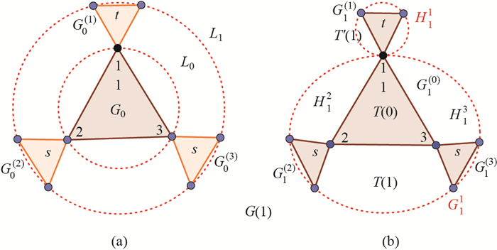
Step 2 Let $G_{0}^{(1)}$ and $G_{0}^{(2, 3)}$ be three copies of $G_0$, whose weighted edges have been scaled by a factor $0 < t < 1$ and $0 < s < 1$, respectively. Let us denote by $p_1^1$ and $p_{2, 3}^{2, 3}$ the nodes in $G_{0}^{(1)}$ and $G_{0}^{(2, 3)}$, respectively, are the image of the initially labeled node $p_i \in G_0$. $G(1)$ is obtained by amalgamating three copies $G_{0}^{(1)}$, $G_{0}^{(2, 3)}$ and $G_0$ by merging three pairs of $p_{1}^{1}$, $p_{2, 3}^{2, 3}$ and $p_i$, $i=1, 2, 3$, respectively, into a new single node which are then the merging nodes $\{p_i:i=1, 2, 3\}$ ($\{1, 2, 3\}$ for short) of $G(1)$, as shown in Figure 6(a).

图 6 (a) The construction of $G(1)$ as layers; (b) $G(1)$ is regarded as the merging of $H_1^1$ and $G_1^1$ Fig.6 (a) The construction of $G(1)$ as layers; (b) $G(1)$ is regarded as the merging of $H_1^1$ and $G_1^1$

For the convenience of constructing $G(2)$, $G(1)$ can also be regarded as the merging of $H_1^1$, $H_1^{2, 3}$ and $G_1^1$, $G_1^{2, 3}$, whose connection nodes are $\{1, 2, 3\}$, respectively, as shown in Figure 6(b). From the self-similarity of $G(1)$, $G(1)$ can be regarded as union of four groups, sequentially denoted as $G_{1}^{(0)}$, $G_{1}^{(1)}$, $G_{1}^{(2)}$ and $G_{1}^{(3)}$.

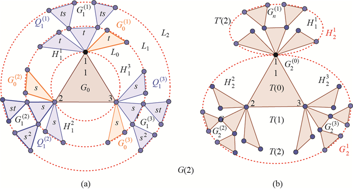
Step 3 Let $G_1^{(1)}$ and $G_1^{(2, 3)}$ be the copy of $G_1^1$ and $G_1^{2, 3}$, whose weighted edges have been scaled by a factor $0 < t < 1$ and $0 < s < 1$, respectively. And let $Q_1^{(1)}=G_1^{(1)}\cup H_1^1$, $Q_1^{(2)}=G_1^{(2)}\cup H_1^2$ and $Q_1^{(3)}=G_1^{(3)}\cup H_1^3$, where $G_1^{(1)}\cap H_1^1=\{p_1^1\}$, $G_1^{(2)}\cap H_1^2=\{p_2^2\}$ and $G_1^{(3)}\cap H_1^3=\{p_3^3\}$, respectively, where $p_1^1$ and $p_{2, 3}^{2, 3}$ are the image of the initially labeled node $\{p_i:i=1, 2, 3\}$. $G(2)$ is obtained by amalgamating three groups $Q_{1}^{(1)}$, $Q_{1}^{(2, 3)}$ and $G(1)$ by merging three pairs of $p_1^1 \in Q_1^{(1)}$, $p_{2, 3}^{2, 3} \in Q_1^{(2, 3)}$ and $p_i \in G(1)$, $i=1, 2, 3$, respectively, into a new single node, which are then the merging nodes $\{p_i:i=1, 2, 3\}$ ($\{1, 2, 3\}$ for short) of $G(2)$, as shown in Figure 7(a).

图 7 (a) The construction of $G(2)$ as layers; (b) $G(2)$ is regarded as the merging of $H_2^1$ and $G_2^1$ Fig.7 (a) The construction of $G(2)$ as layers; (b) $G(2)$ is regarded as the merging of $H_2^1$ and $G_2^1$

For the convenience of constructing $G(3)$, $G(2)$ can be regarded as the merging of $H_2^1$, $H_2^{2, 3}$ and $G_2^1$, $G_2^{2, 3}$, whose connection nodes are $\{1, 2, 3\}$, respectively, as shown in Figure 7(b). From the self-similarity of $G(2)$, $G(2)$ can be regarded as the union of four groups, sequentially denoted as $G_{2}^{(0)}$, $G_{2}^{(1)}$, $G_{2}^{(2)}$ and $G_{2}^{(3)}$.

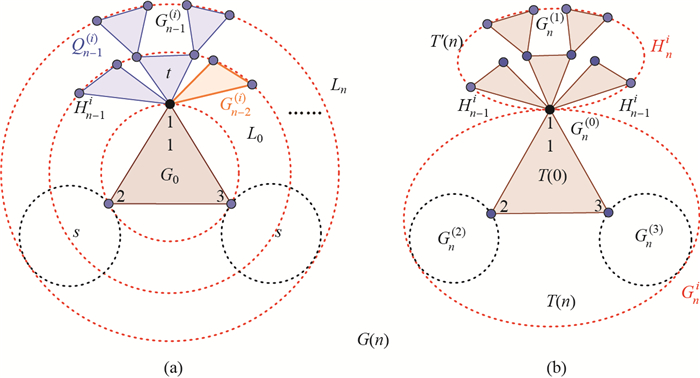
Step n A large network of order $k=n+1$ is obtained as follows. Firstly, for the convenience of constructing $G(n+1)$, $G(n)$ can be regarded as the merging of $H_n^1$, $H_n^{2, 3}$ and $G_n^1$, $G_n^{2, 3}$, whose connection nodes are $\{1, 2, 3\}$, respectively, as shown in Figure 8(b). From the self-similarity of $G(n)$, $G(n)$ can be regarded as four groups, sequentially denoted as $G_{n}^{(0)}$, $G_{n}^{(1)}$, $G_{n}^{(2)}$ and $G_{n}^{(3)}$. One group is $G_{n}^{(0)}=G_0-\{p_i:i=1, 2, 3\}$; then $G(n)-G_{n}^{(0)}$ consists of the same three disjoint groups $G_{n}^{(1)}$ and $G_{n}^{(2, 3)}$, whose merging node is linked to the corresponding initial merging node $p_i$ of $G_0$. Let $G_n^i=(G(n)-H_n^i)\cup \{p_i\}$, $i=1, 2, 3$; then $H_n^i\cap G_n^i=\{p_i\}$, $i=1, 2, 3$.

图 8 (a) The construction of $G(n)$ as layers; (b) $G(n)$ is regarded as the merging of $H_n^i$ and $G_n^i$ Fig.8 (a) The construction of $G(n)$ as layers; (b) $G(n)$ is regarded as the merging of $H_n^i$ and $G_n^i$

Secondly, let $G_{n-1}^{(1)}$ and $G_{n-1}^{(2, 3)}$ be the copy of $G_{n-1}^1$ and $G_{n-1}^{2, 3}$, whose weighted edges have been scaled by a factor $0 < t < 1$ and $0 < s < 1$, respectively. Let $Q_{n-1}^{(1)}=G_{n-1}^{(1)}\cup H_{n-1}^1$, $Q_{n-1}^{(2)}=G_{n-1}^{(2)}\cup H_{n-1}^2$ and $Q_{n-1}^{(3)}=G_{n-1}^{(3)}\cup H_{n-1}^3$, where $G_{n-1}^{(1)}\cap H_{n-1}^1=\{p_1^1\}$, $G_{n-1}^{(2)}\cap H_{n-1}^2=\{p_2^2\}$ and $G_{n-1}^{(3)}\cap H_{n-1}^3=\{p_3^3\}$, respectively, where $p_1^1$ and $p_{2, 3}^{2, 3}$ are the image of the initially labeled node $\{p_i:i=1, 2, 3\}$.

Finally, $G(n)$ is obtained by amalgamating three groups $Q_{n-1}^{(1)}$, $Q_{n-1} ^{(2, 3)}$ and $G(n-1)$ and by merging three pairs of $p_1^1 \in Q_{n-1}^{(1)}$, $p_{2, 3}^{2, 3} \in Q_{n-1}^{(2, 3)}$ and $p_i \in G(n-1)$, $i=1, 2, 3$, respectively, into a new single node which are then the merging nodes $\{p_i:i=1, 2, 3\}$ ($\{1, 2, 3\}$ for short) of $G(n)$, as shown in Figure 8. Hence, a recursive non-homogeneous weighted Koch network created by the recursive division method was obtained.

4 Average weighted receiving time for scaling factors t, s

We use the same basic definitions given in Section 2 for all quantities and concepts in this section. $\langle T \rangle_k$ is the average non-homogeneous weighted receiving time (AN-HWRT), which is defined in Eq (2.4) as the average of $F_j(k)$ over all starting nodes $j\in G(k)=H_k^1\cup H_k^{2, 3}$, where $H_k^1\cap H_k^{2, 3}=\{1\}$ other than the trap in $G(0)$.

4.1 Recurrence formula of $T_{\rm tot}(k)$ for scaling factors $t, s$

For a large network from the graph, we can obtain the formulas of $T^{\prime}(k)$ and $T(k)$ by the transition from $G(n-1)$ to $G(n)$.

The group $H_n^1$ of graph $G(n)$ consists of the union of three disjoint groups $G_{n-2}^{(1)}, G_{n-2}^{(1)}$ and $G_{n-1}^{(1)}$; then $H_n^1=G_{n-2}^{(1)}\cup G_{n-2}^{(1)}\cup G_{n-1}^{(1)}$, where $G_{n-1}^{(1)}=tT(n-1)$ and $G_{n-2}^{(1)}=T^{\prime}(n-1)$. From the definition of $T^{\prime}(n)$, we obtain

$ \begin{equation*} T^{\prime}(n)=2T^{\prime}(n-1)+tT(n-1). \end{equation*} $ (4.1)

The group $H_n^{2, 3}$ of graph $G(n)$ consists of the union of three disjoint groups $2sG_{n-2}^{(1)}, sG_{n-2}^{(2, 3)}$ and $2G_{n-2}^{(2, 3)}$; then $H_n^{2, 3}=2sG_{n-2}^{(1)} \cup sG_{n-2}^{(2, 3)} \cup 2G_{n-2}^{(2, 3)}$ and these three groups are obtained as $2sG_{n-2}^{(1)}=2sT^\prime(n-1)+\frac{2}{3}(2s+2)N_{n-1}$, $sG_{n-2}^{(2, 3)}=sT(n-1)+2(\frac{2}{3}N_{n-1})$ and $2G_{n-2}^{(2, 3)}=2T(n-1)-4$. From the definition of $T(n)$, we obtain

$ \begin{equation*} T(n)=2sT^{\prime}(n-1)+(s+2)T(n-1)+\dfrac{4}{3}sN_{n-1}+\dfrac{8}{3}N_{n-1}-4. \end{equation*} $ (4.2)

See Figure 9. If we fix $k=n$, we can rewrite Eq (4.1) and Eq (4.2) in the form

$ \begin{equation*} K_n=AK_{n-1}+\alpha(n), \end{equation*} $ (4.3)
图 9 (a) The construction of $G(n-1)$; (b) The construction of $G(n)$ Fig.9 (a) The construction of $G(n-1)$; (b) The construction of $G(n)$

where $K_n= \begin{pmatrix} T^\prime(n) \\T(n)\end{pmatrix}$, $A= \begin{pmatrix} 2&t \\ 2s&s+2 \end{pmatrix}$, $\alpha(n)= \begin{pmatrix} 0 \\a_n \end{pmatrix}$ and $a_n=\frac{4}{3}sN_{n-1}+\frac{8}{3}N_{n-1}-4$. We can solve Eq (4.3) inductively to get

$ \begin{equation*} K_n=A^nK_{0}+\sum\limits_{i=1}^{n}A^{n-i}\alpha(i). \end{equation*} $ (4.4)

Now, by using singular value decomposition in this work, we seek to find the eigenvalues and the eigenvectors of the matrix $A_{2\times2}$ which represents a linear transformation. For this matrix, there are two eigenvalues equivalent to the two roots of the equation $\lambda^2-(\textrm{tr}A)\lambda+\textrm{det}A=0$; the two eigenvalues are $\lambda_1=\frac{s+4+\alpha}{2}$ and $\lambda_2=\frac{s+4-\alpha}{2}$, where $\alpha=\sqrt{s^2+8ts}$. Thus, we get two non-zero eigenvectors satisfying $Av_i=\lambda_iv_i, i=1, 2$, $v_1=\begin{pmatrix} 2t \\s+\alpha \end{pmatrix}$ and $v_2=\begin{pmatrix} 2t \\s-\alpha \end{pmatrix}$ corresponding to $\lambda_1$ and $\lambda_2$. So we can rewrite matrix $A$ as $A=V \Sigma V^{-1}$, where $V= \begin{pmatrix} 2t&2t \\ s+\alpha&s-\alpha\end{pmatrix}$, $\Sigma= \begin{pmatrix} \frac{s+4+\alpha}{2}&0 \\ 0&\frac{s+4-\alpha}{2}\end{pmatrix}$ and $V^{-1}=\frac{-1}{4t\alpha} \begin{pmatrix} s-\alpha&-2t \\ -(s+\alpha)&2t\end{pmatrix}$; then we have

$ A^{n}= \begin{pmatrix} 2&t \\ 2s&s+2 \end{pmatrix}^{n} \\ =\begin{pmatrix} \dfrac{-(s-\alpha)}{2\alpha}\left(\dfrac{s+4+\alpha}{2}\right)^{n}+ \dfrac{(s+\alpha)}{2\alpha}\left(\dfrac{s+4-\alpha}{2}\right)^{n}& \dfrac{t}{\alpha}\left(\dfrac{s+4+\alpha}{2}\right)^{n} -\dfrac{t}{\alpha}\left(\dfrac{s+4-\alpha}{2}\right)^{n} \\[3mm] \dfrac{-(s^2-\alpha^2)}{4t\alpha}\left(\dfrac{s+4+\alpha}{2}\right)^{n}+ \dfrac{(s^2-\alpha^2)}{4t\alpha}\left(\dfrac{s+4-\alpha}{2}\right)^{n}& \dfrac{(s+\alpha)}{2\alpha}\left(\dfrac{s+4+\alpha}{2}\right)^{n}- \dfrac{s-\alpha}{2\alpha}\left(\dfrac{s+4-\alpha}{2}\right)^{n} \end{pmatrix}. $ (4.5)

By using $K_0= \begin{pmatrix} T^\prime(0) \\ T(0)\end{pmatrix}=\begin{pmatrix} 0 \\ 4\end{pmatrix}$ for the initial network and based on Eq (4.5), we obtain

$ A^nK_0\!=\! \left(\!\! {{\begin{array}{*{20}c}\dfrac{4t}{\alpha} \left(\dfrac{s+4+\alpha}{2}\right)^{n}\!-\! \dfrac{4t}{\alpha}\left(\dfrac{s+4-\alpha}{2}\right)^{n} \\[4mm] \dfrac{2(s+\alpha)}{\alpha}\left(\dfrac{s+4+\alpha}{2}\right)^{n} \!-\!\dfrac{2(s-\alpha)}{\alpha}\left(\dfrac{s+4-\alpha}{2}\right)^{n} \end{array}}}\!\! \right) $

and

$ \sum\limits_{i=1}^{n}A^{n-i}\alpha(i)= \begin{pmatrix} \dfrac{t}{\alpha}\sum\limits_{i=1}^{n}\left(\dfrac{s+4+\alpha}{2}\right) ^{n-i}a_i-\dfrac{t}{\alpha}\sum\limits_{i=1}^{n}\left(\dfrac{s+4-\alpha}{2}\right)^{n-i}a_i \\[3mm] \dfrac{s+\alpha}{2\alpha}\sum\limits_{i=1}^{n}\left(\dfrac{s+4+ \alpha}{2}\right)^{n-i} a_i-\dfrac{(s-\alpha)}{2\alpha}\sum\limits_{i=1}^{n} \left(\dfrac{s+4-\alpha}{2}\right)^{n-i}a_i \end{pmatrix}. $

From Eq (4.4) we get

$ K_n\!=\! \begin{pmatrix} \dfrac{4t}{\alpha}\left(\left(\dfrac{s+4+\alpha}{2}\right)^{n} \!-\!\left(\dfrac{s+4-\alpha}{2}\right)^{n}\right) \!+\!\dfrac{t}{\alpha}\Big(\sum\limits_{i=1}^{n} \left(\dfrac{s+4+\alpha}{2}\right)^{n-i} a_i\!-\!\sum\limits_{i=1}^{n}\left(\dfrac{s+4-\alpha}{2}\right)^{n-i}a_i\Big) \\[3mm] \dfrac{2}{\alpha}\left((s+\alpha)\left(\dfrac{s+4+\alpha}{2}\right)^{n} \!-\!(s-\alpha)\left(\dfrac{s+4-\alpha}{2}\right)^{n}\right) \!+\! \dfrac{1}{2\alpha}\Big((s+\alpha)\sum\limits_{i=1}^{n} \left(\dfrac{s+4+\alpha}{2}\right)^{n-i} a_i\!-\!(s-\alpha)\sum\limits_{i=1}^{n} \left(\dfrac{s+4-\alpha}{2}\right)^{n-i}a_i\Big) \end{pmatrix}. $

Then, we obtain the formula of $T^\prime(n)$ and $T(n)$ as follows

$ \begin{align*} T^\prime(n)=&\dfrac{4t}{\alpha}\left(\left(\dfrac{s+4+\alpha}{2}\right)^{n} -\left(\dfrac{s+4-\alpha}{2}\right)^{n}\right) \nonumber\\ &+\dfrac{t}{\alpha}\left(\sum\limits_{i=1}^{n}\left(\dfrac{s+4+\alpha}{2}\right)^{n-i}a_i-\sum\limits_{i=1}^{n}\left(\dfrac{s+4-\alpha}{2}\right)^{n-i}a_i\right) \end{align*} $ (4.6)

and

$ \begin{align*} T(n)=&\dfrac{2}{\alpha}\left((s+\alpha)\left(\dfrac{s+4+\alpha}{2}\right)^{n}-(s-\alpha)\left(\dfrac{s+4-\alpha}{2}\right)^{n}\right) \nonumber\\ &+ \dfrac{1}{2\alpha}\left((s+\alpha)\sum\limits_{i=1}^{n}\left(\dfrac{s+4+\alpha}{2}\right)^{n-i}a_i-(s-\alpha)\sum\limits_{i=1}^{n}\left(\dfrac{s+4-\alpha}{2}\right)^{n-i}a_i\right). \end{align*} $ (4.7)

From the definition of $T_{\rm tot}(n)$, we can write $T_{\rm tot}(n)$ as

$ \begin{align*} T_{\rm tot}(n)= &\dfrac{4t+2(s+\alpha)}{\alpha}\left(\dfrac{s+4+\alpha}{2}\right)^{n}-\left(\dfrac{4t+2(s-\alpha)}{\alpha}\right)\left(\dfrac{s+4-\alpha}{2}\right)^{n}\\ &+\dfrac{2t+s+\alpha}{2\alpha}\sum\limits_{i=1}^{n}\left(\dfrac{s+4+\alpha}{2}\right)^{n-i}a_i-\left(\dfrac{2t+s-\alpha}{2\alpha}\right)\sum\limits_{i=1}^{n}\left(\dfrac{s+4-\alpha}{2}\right)^{n-i}a_i, \end{align*} $

where $a_i=\frac{4}{3}sN_{i-1}+\frac{8}{3}N_{i-1}-4$ and $N_{i-1}=2\times 4^{i-1}+1$; then $a_i=\frac{2}{3}(s+2)4^i+\frac{4}{3}(s-1)$. Accordingly, we have

$ \begin{array}{l} {T_{{\rm{tot}}}}(n) = \frac{1}{{{2^n}}}((4t + 2s + 2\alpha ){(s + 4 + \alpha )^n} - (4t + 2s - 2\alpha ){(s + 4 - \alpha )^n})\;\;\;\;\;\;\;\;\;\;\;\\ \;\;\;\;\;\;\;\;\;\;\;\; - \frac{{(2t + s + \alpha )}}{{3 \times {2^{n - 2}}\alpha }}\left( {\frac{{2(s + 2)({8^n} - {{(s + 4 + \alpha )}^n})}}{{s - 4 + \alpha }} + \frac{{(s - 1)({2^n} - {{(s + 4 + \alpha )}^n})}}{{s + 2 + \alpha }}} \right)\;\;\;\;\;\;\;\;\;\;\;\\ \;\;\;\;\;\;\;\;\;\;\;\; + \frac{{(2t + s - \alpha )}}{{3 \times {2^{n - 2}}\alpha }}\left( {\frac{{2(s + 2)({8^n} - {{(s + 4 - \alpha )}^n})}}{{s - 4 - \alpha }} + \frac{{(s - 1)({2^n} - {{(s + 4 - \alpha )}^n})}}{{s + 2 - \alpha }}} \right). \end{array} $ (4.8)
4.2 Formula of $\langle T \rangle_k$ for scaling factors $t, s$

Finally, recalling $N_k=2\times 4^k+1$ and using Eq (4.8), we can work out from the definition of $\langle T \rangle_k$ the expression of $T_{\rm tot}(k)$ in Eq (2.3), for any $k=0, 1, 2, \cdots, n$:

$ \begin{align*} \langle T \rangle_k= &\dfrac{1}{2^{3k+1}\alpha}\left((4t+2s+2\alpha)(s+4+\alpha)^k-(4t+2s-2\alpha)(s+4-\alpha)^k\right) \\[2mm] &-\dfrac{(2t+s+\alpha)}{3\times 2^{3k-1}\alpha}\left(\dfrac{2(s+2)(8^k-(s+4+\alpha)^k)}{s-4+\alpha}+\dfrac{(s-1)(2^k-(s+4+\alpha)^k)}{s+2+\alpha}\right) \\[2mm] &+\dfrac{(2t+s-\alpha)}{3\times 2^{3k-1}\alpha}\left(\dfrac{2(s+2)(8^k-(s+4-\alpha)^k)}{s-4-\alpha}+\dfrac{(s-1)(2^k-(s+4-\alpha)^k)}{s+2-\alpha}\right). \end{align*} $ (4.9)

For a large network, the AN-HWRT grows as a constant of the network order when the $k$-th generation goes to infinity; then $\langle T \rangle_k$ can be obtained as

$ \langle T \rangle_k \approx \dfrac{2\times 8^k(s+2)(2t+s-\alpha)}{3\times 2^{-1}\times 2^{3k}\alpha(s-4-\alpha)} -\dfrac{2\times 8^k(s+2)(2t+s+\alpha)}{3\times 2^{-1}\times 2^{3k}\alpha(s-4+\alpha)}. $

Hence for $0<t, s<1$, $\langle T \rangle_k$ can be obtained as the constant

$ \begin{equation} \langle T \rangle_k=\dfrac{16(t+2)(s+2)}{3(16-8s(t+1))}. \end{equation} $ (4.10)
5 Non-homogenous weighted Koch networks created by the recursive division method for different scaling factors

Given the non-homogeneous weighted Koch network is developed in [17], with three scaling factors $t, r, s\in(0, 1)$ instead of two scaling factors $t, s\in(0, 1)$, and the weighted tetrahedron Koch networks is developed in [14], we can introduce a family of non-homogeneous weighted Koch networks on a random walk, where the average weighted receiving time (AWRT) was defined in [17].

Inspired by metabolic networks and airport networks, we introduce recursive non-homogeneous weighted Koch networks in which each edge weight in every triangle is related to the triangle's topology and depends on the scaling factors $0 < t$, $r$, and $s < 1$. In these networks, we follow the same topology of the triangle, where the three edges have the same weight and the same processes of construction as the recursive formulas of non-homogeneous weighted Koch networks described in Sections 1 and 3. As mentioned above, we will use the recursive division method to define recursive non-homogeneous weighted Koch networks. Let us fix three positive real numbers $t$, $r$, $s(\in(0, 1))$.

6 Average weighted receiving time for scaling factors $t, r, s$

We follow the same basic definitions given in Section 2 for all quantities and concepts in this section. $\langle T \rangle_k$ is the average non-homogeneous weighted receiving time (AN-HWRT), which is defined by Eq (2.4) as the average of $F_j(k)$ over all starting nodes $j\in G(k)=H_k^1\cup H_k^2\cup H_k^3$, where $H_k^1\cap (H_k^2\cup H_k^3)=\{1\}$ other than the trap in $G(0)$.

Here, we denote by $T_1(k)$, the sum of MWLPs of all nodes in $H_k^1$ absorbed at the trap located at the merging node $p_1\in L_0$ of $G(k)$, i.e., $T_1(k)=\sum_{j\in H_k^1\setminus\{1\}}F_j(k)$, denoted by $T_2(k)$ as the sum of MWLPs of all nodes in $H_k^2$ absorbed at the trap located in the merging node $p_1\in L_0$ of $G(k)$. Hence, $T_2(k)=\sum_{j\in H_k^2\setminus\{1\}}F_j(k)$ denoted by $T_3(k)$ as the sum of MWLPs of all nodes in $H_k^3$ absorbed at the trap located in the merging node $p_1\in L_0$ of $G(k)$, i.e.,

$T_3(k)=\sum_{j\in H_k^3\setminus\{1\}}F_j(k)$. Then we can denote by $T_{\rm tot}(k)$, the sum of MWLPs of all nodes in $G(k)=H_k^1\cup H_k^2\cup H_k^3$ absorbed at the trap located at the merging node $p_1\in L_0$ of $G(k)$, i.e.,

$ \begin{equation} T_{\rm tot}(k)=T_1(k)+T_2(k)+T_3(k)=\sum\limits_{n=1}^{3}T_n(k)=\sum\limits_{j\in G(k)\setminus\{1\}}F_j(k). \end{equation} $ (6.1)

Now, $\langle T \rangle_k$ is the average non-homogeneous weighted receiving time (AN-HWRT), which is defined as the average of $F_j(k)$ over all starting nodes $j\in G(k)=H_k^1\cup H_k^2\cup H_k^3$, where $H_k^1\cap (H_k^2\cup H_k^3)=\{1\}$ other than the trap in $G(0)$; then we have

$ \begin{equation}\label{E:6.2} \langle T \rangle_k=\dfrac{T_{\rm tot}(k)}{N_k-1}. \end{equation} $ (6.2)

Thus, the problem of determining $\langle T \rangle_k$ is reduced to finding $T_{\rm tot}(k)$. By the construction of $G(k)$, $G(k)$ can also be regarded as the merging of $H_k^1$, $H_k^2$ and $H_k^3$, whose merging nodes are $p_i\in L_0, i=1, 2, 3$.

6.1 Recurrence formula of $T_{\rm tot}(k)$ for scaling factors $t, r, s$

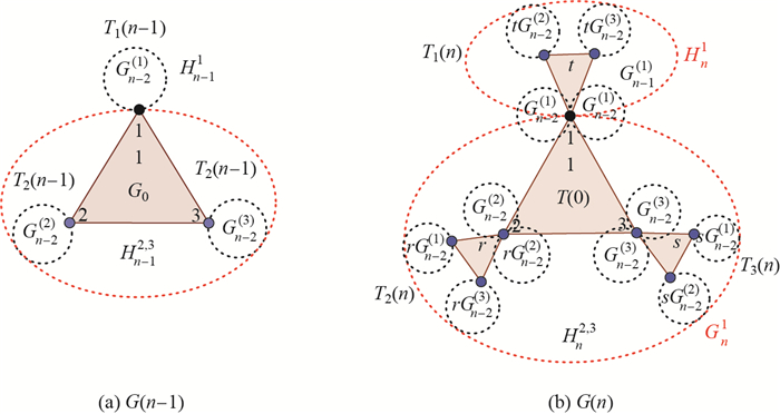
For a large network, from the graph, we can obtain the formulas of $T_1(k)$, $T_2(k)$ and $T_3(k)$ by the transition from $G(n-1)$ to $G(n)$. The group $H_n^1$ of the graph $G(n)$ consists of the union of three disjoint groups $G_{n-2}^{(1)}, G_{n-2}^{(1)}, G_{n-1}^{(1)}$; then $H_n^1=G_{n-2}^{(1)}\cup G_{n-2}^{(1)}\cup G_{n-1}^{(1)}$, where $G_{n-1}^{(1)}=tT_2(n-1)+tT_3(n-1)$ and $G_{n-2}^{(1)}=T_1(n-1)$. From the definition of $T_1(n)$ we obtain

$ T_1(n)=2T_1(n-1)+tT_2(n-1)+tT_3(n-1). $ (6.3)

The group $H_n^2$ of the graph $G(n)$ consists of the union of three disjoint groups $rG_{n-2}^{(1)}, 2G_{n-2}^{(2)}$ and $rG_{n-2}^{(3)}$; then $H_n^2=rG_{n-2}^{(1)} \cup 2G_{n-2}^{(2)} \cup rG_{n-2}^{(3)}$. These three groups are obtained as $rG_{n-2}^{(1)}=rT_1(n-1)+\frac{1}{3}(2r+2)N_{n-1}$, $2G_{n-2}^{(2)}=2T_2(n-1)-2$ and $rG_{n-2}^{(3)}=rT_3(n-1)+\frac{2}{3}N_{n-1}$; from the definition of $T_2(n)$ we obtain

$ \begin{equation} T_2(n)=rT_1(n-1)+2T_2(n-1)+rT_3(n-1)+\dfrac{2}{3}rN_{n-1}+\dfrac{4}{3}N_{n-1}-2. \end{equation} $ (6.4)

The group $H_n^3$ of the graph $G(n)$ consists of the union of three disjoint groups $sG_{n-2}^{(1)}, sG_{n-2}^{(2)}$ and $2G_{n-2}^{(3)}$; then $H_n^3=sG_{n-2}^{(1)} \cup sG_{n-2}^{(2)} \cup 2G_{n-2}^{(3)}$. These three groups are obtained as $sG_{n-2}^{(1)}=sT_1(n-1)+\dfrac{1}{3}(2s+2)N_{n-1}$, $sG_{n-2}^{(2)}=sT_2(n-1)+\dfrac{2}{3}N_{n-1}$ and $2G_{n-2}^{(3)}=2T_3(n-1)-2$; from the definition of $T_3(n)$ we obtain

$ \begin{equation} T_3(n)=sT_1(n-1)+sT_2(n-1)+2T_3(n-1)+\dfrac{2}{3}sN_{n-1}+\dfrac{4}{3}N_{n-1}-2. \end{equation} $ (6.5)

See Figure 10.

图 10 (a) The construction of $G(n-1)$; (b) the construction of $G(n)$ Fig.10 (a) The construction of $G(n-1)$; (b) the construction of $G(n)$

If we fix $k=n$, we can rewrite Eq (6.3), Eq (6.4) and Eq (6.5) in the form

$ \begin{equation} K_n=AK_{n-1}+\alpha(n), \end{equation} $ (6.6)

where $K_n= \begin{pmatrix} T_1(n) \\T_2(n) \\T_3(n) \end{pmatrix}$, $A= \begin{pmatrix} 2&t&t \\ r&2&r \\ s&s&2 \end{pmatrix}$, $\alpha(n)= \begin{pmatrix} a_n \\b_n \\c_n \end{pmatrix}$, $a_n=0$, $b_n=\frac{2}{3}rN_{n-1}+\frac{4}{3}N_{n-1}-2$ and $c_n=\frac{2}{3}sN_{n-1}+\frac{4}{3}N_{n-1}-2$. We can solve the equation Eq (6.6) inductively to get

$ \begin{equation} K_n=A^nK_{0}+\sum\limits_{i=1}^{n}A^{n-i}\alpha(i). \end{equation} $ (6.7)

By using singular value decomposition, the matrix of the form $A_{3\times3}$ which represents a linear transformation with three eigenvalues $\lambda_1$, $\lambda_2$ and $\lambda_3$ is equivalent to the three roots of the equation $\lambda^3-6\lambda^2-(rs+tr+ts-12)\lambda+2(rs+tr+ts-trs-4)=0$. Thus, we have three non-zero eigenvectors satisfying $Av_i=\lambda_iv_i, i=1, 2, 3$ corresponding to the eigenvalues $\lambda_1$, $\lambda_2$ and $\lambda_3$, respectively. We can rewrite matrix $A$ as $A=V \Sigma V^{-1}$, where $\Sigma= \begin{pmatrix} \lambda_1&0&0 \\ 0&\lambda_2&0 \\ 0&0 & \lambda_3 \end{pmatrix}$ and $V$ is the matrix of the eigenvectors, then we have

$ A^{n}= \begin{pmatrix} 2 & t & t \\ r & 2 & r \\ s & s & 2 \end{pmatrix}^{n} =V \begin{pmatrix} \lambda_1^{n} & 0 & 0 \\ 0 & \lambda_2^{n} & 0 \\ 0 & 0 & \lambda_3^{n} \end{pmatrix}V^{-1}. $ (6.8)

Researchers can study the last case further and extract the exact formulas $T_{\rm tot}(k)$ and $\langle T \rangle_k$ for three different parameters $0 < t, r, s < 1$, in the large networks, average weighted receiving time (AWRT) $\langle T \rangle_k$ grows with $\theta(t, r, s)$.

7 Conclusions

In this work, we have addressed the topic of recursive homogeneous and non-homogeneous weighted Koch networks, where the edges carry the weights of their respective nodes to a given fixed target node. Although such networks appear at first to be substantially more difficult to understand than their unweighted counterparts, we have shown that in many cases recurrence graphs are commonly the best way to understand large and complex networks. The methods presented in this paper, such as the recursive division method, are intended for the study of weighted networks, which are regard as a guide for thinking about such systems. We look forward with interest to learning about other applications of these ideas. Finally, we have discussed the impact of the key parameter $0 < t < 1$ for the homogeneous model and $0 < t, s < 1$ or $0 < t, r, s < 1$ for non-homogeneous models on AWRT. Our analysis indicates that in a large network, the AWRT grows as a constant of the network order when the $k$-th generation goes to infinity; this is represented by $\theta(t)=\frac{2(t+2)}{3(1-t)}, 0 < t< 1$ for the homogeneous model and by $\theta(t, s)=\frac{16(s+2)(t+2)}{3(16-8s(t+1))}, 0 < t, s< 1$ for the non-homogeneous model. In the next work, we will derive an explicit formula for AWRT with three different parameters $0 < t, r, s < 1$ and grows with $\theta(t, r, s)$.

Acknowledgements

The authors would like to thank Prof. Wenxia Li and Dr. Junjie Miao for the useful discussions.

参考文献
[1]
FRIEZE A, KARONSKI M. Introduction to Random Graphs[M]. Cambridge: Cambridge University Press, 2015.
[2]
CIEPLAK M, GIACOMETTI A, MARITAN A, et al. Models of fractal river basins[J]. Journal of Statistical Physics, 1998, 91(1/2): 1-15. DOI:10.1023/A:1023069201470
[3]
ZHAO L, LAI Y C, PARK K, et al. Onset of traffic congestion in complex networks[J]. Phys Rev E Stat Nonlin Soft Matter Phys, 2005, 71(2): 026125. DOI:10.1103/PhysRevE.71.026125
[4]
GARlASCHELLI D, LOFFREDO M I. Fitness-dependent topological properties of the world trade web[J]. Physical Review Letters, 2004, 93(18): 188701. DOI:10.1103/PhysRevLett.93.188701
[5]
GUIMERA R, AMARAL L A N. Modeling the world-wide airport network[J]. European Physical Journal B, 2004, 38(2): 381-385. DOI:10.1140/epjb/e2004-00131-0
[6]
MACDONALD P J, ALMAAS E, BARABASI A L. Minimum spanning trees of weighted scale-free networks[J]. Epl, 2005, 72(2): 308-314. DOI:10.1209/epl/i2005-10232-x
[7]
DAI M, SUN Y, SHAO S, et al. Modified box dimension and average weighted receiving time on the weighted fractal networks[J]. Scientific Reports, 2015, 5: 18210.
[8]
WEI D J, LIU Q, ZHANG H X, et al. Box-covering algorithm for fractal dimension of weighted networks[J]. Sci Rep, 2013, 3(6157): 3049.
[9]
CARLETTI T. Stochastic weighted fractal networks[J]. Physics, 2012, 389(10): 2134-2142.
[10]
CARLETTI T, RIGHI S. Weighted fractal networks[J]. Physica A, 2009, 389(10): 2134-2142.
[11]
YUAN Z J, GANG S W, RONG C G. Exact scaling for the mean first-passage time of random walks on a generalized Koch network with a trap[J]. Chinese Physics B, 2012, 21(3): 525-529.
[12]
LI L, SUN W G, WANG G X, et al. Mean first-passage time on a family of small-world treelike networks[J]. International Journal of Modern Physics C, 2014, 25(3): 1350097(10 pages).
[13]
ZHANG Z, GAO S. Scaling of mean first-passage time as efficiency measure of nodes sending information on scale-free Koch networks[J]. The European Physical Journal B, 2011, 80(2): 209-216. DOI:10.1140/epjb/e2011-10863-1
[14]
DAI M F, XIE Q, XI L F. Trapping on weighted tetrahedron Koch networks with small-world property[J]. Fractals, 2014, 22(1/2): 1450006(9 pages). https: //www.researchgate.net/publication/263906960_Trapping_on_weighted_tetrahedron_koch_networks_with_small-world_property
[15]
SUN W. Random walks on generalized Koch networks[J]. Physica Scripta, 2013, 88(4): 045006. DOI:10.1088/0031-8949/88/04/045006
[16]
DAI M F, YE D D, LI X Y, et al. Average weighted receiving time in recursive weighted Koch networks[J]. Pramana, 2016, 86(6): 1173-1182. DOI:10.1007/s12043-016-1196-8
[17]
DAI M F, LI X Y, XI L F. Random walks on non-homogenous weighted Koch networks[J]. Chaos:An Interdisciplinary Journal of Nonlinear Science, 2013, 23(3): 033106. DOI:10.1063/1.4810927
[18]
DONG Y, DAI M, YE D. Non-homogeneous fractal hierarchical weighted networks[J]. Plos One, 2015, 10(4): e0121946. DOI:10.1371/journal.pone.0121946